The Legend of Shannon’s Entropy

Posted Sep 2, 2026

The fundamental problem of communication is that of reproducing at one point either exactly or approximately a message selected at another point. - Claude Shannon

By Keyur Ramoliya

70 min read

The Legend of Shannon’s Entropy

Every GPT-style language model is trained with the same objective. The transformer takes a context of tokens, the last layer maps that representation onto the vocabulary, and a softmax turns the scores into a probability distribution over the next token (Vaswani et al., 2017; Radford et al., 2018). The loss is the cross-entropy between that distribution and the token that actually appeared. If the model assigned probability $q$ to the true next token, the loss on that step is $-\log q$ (Radford et al., 2018). Average it over a corpus and you have a rate, in bits or nats per token, of how surprised the model is by the data.

That number is not a neural-network invention. Cross-entropy is Shannon’s entropy of the true next-token distribution, plus the extra surprise that comes from using the wrong probabilities. When the model matches the data, the extra term vanishes and the training loss equals the entropy of the source. A GPT architecture is, in Shannon’s language, a statistical approximation to English, trained to approach the entropy of the source (Radford et al., 2018; Radford et al., 2019). He built the first rungs of that ladder by hand in 1948, with letter frequencies, then digrams, then words (Shannon, 1948, Section 3). The transformer is the same idea at a scale he did not have.

The paper that defined that entropy is Claude Shannon’s A Mathematical Theory of Communication, published in two parts in the Bell System Technical Journal in 1948 (Shannon, 1948; Tse, 2020). A basis for such a theory is contained in the important papers of Nyquist and Hartley on this subject (Shannon, 1948, Introduction; Nyquist, 1924; Nyquist, 1928; Hartley, 1928). In the present paper we will extend the theory to include a number of new factors, in particular the effect of noise in the channel, and the savings possible due to the statistical structure of the original message and due to the nature of the final destination of the information (Shannon, 1948, Introduction). This means the paper is not only about how many signals a wire can carry. It is about what the source looks like statistically, what noise does to those signals, and what the destination actually needs recovered.

The Communication System Shannon Defined

Meaning Is Not the Engineering Problem

The fundamental problem of communication is that of reproducing at one point either exactly or approximately a message selected at another point (Shannon, 1948, Introduction). That sentence is the whole field in one line. Communication is selection and reproduction, not understanding.

Frequently the messages have meaning; that is they refer to or are correlated according to some system with certain physical or conceptual entities. These semantic aspects of communication are irrelevant to the engineering problem (Shannon, 1948, Introduction). This means a telephone circuit does not need to know whether the waveform is a stock price or a poem. It needs to know how to put the selected waveform back together at the other end. Weaver later split the problem into technical, semantic, and effectiveness levels; Shannon’s theory is the first of those (Weaver, 1949).

The significant aspect is that the actual message is one selected from a set of possible messages. The system must be designed to operate for each possible selection, not just the one which will actually be chosen since this is unknown at the time of design (Shannon, 1948, Introduction). If the set is finite and all choices are equally likely, this number or any monotonic function of this number can be regarded as a measure of the information produced when one message is chosen from the set (Shannon, 1948, Introduction). As was pointed out by Hartley the most natural choice is the logarithmic function (Shannon, 1948, Introduction; Hartley, 1928). This means information is how large the set of possible messages is, not how important any one message is, and the log turns that size into something that adds when you add hardware.

Why the Logarithm, and What a Bit Is

The logarithmic measure is more convenient for various reasons (Shannon, 1948, Introduction). The three reasons that follow are engineering, intuition, and algebra, not a claim about meaning.

It is practically more useful. Parameters of engineering importance such as time, bandwidth, number of relays, etc., tend to vary linearly with the logarithm of the number of possibilities (Shannon, 1948, Introduction). For example, adding one relay to a group doubles the number of possible states of the relays. It adds 1 to the base 2 logarithm of this number (Shannon, 1948, Introduction). Doubling the time roughly squares the number of possible messages, which doubles the logarithm. This means the quantities you actually pay for, time, bandwidth, hardware, scale with bits, not with the raw count of messages.

It is nearer to our intuitive feeling as to the proper measure (Shannon, 1948, Introduction). One feels, for example, that two punched cards should have twice the capacity of one for information storage, and two identical channels twice the capacity of one for transmitting information (Shannon, 1948, Introduction). Capacity should add when you add hardware. Only the logarithm does that.

It is mathematically more suitable. Many of the limiting operations are simple in terms of the logarithm but would require clumsy restatement in terms of the number of possibilities (Shannon, 1948, Introduction). Sums, limits, and rates stay linear in bits. They would be messy if you tracked the size of the set directly.

The choice of a logarithmic base corresponds to the choice of a unit for measuring information (Shannon, 1948, Introduction). If the base 2 is used the resulting units may be called binary digits, or more briefly bits, a word suggested by J. W. Tukey (Shannon, 1948, Introduction). A device with two stable positions, such as a relay or a flip-flop circuit, can store one bit of information. $N$ such devices can store $N$ bits, since the total number of possible states is $2^N$ and $\log_2 2^N = N$ (Shannon, 1948, Introduction). An $N$-bit register has exactly $2^N$ states, so the unit matches the hardware.

If the base 10 is used the units are decimal digits, with

\[\log_2 M = \frac{\log_{10} M}{\log_{10} 2} \approx 3.32 \log_{10} M\]

so a decimal digit is about $3\frac{1}{3}$ bits (Shannon, 1948, Introduction). In analytical work where integration and differentiation are involved the base $e$ is sometimes useful. The resulting units of information will be called natural units (Shannon, 1948, Introduction). Change of base is multiplication by $\log_b a$. Nats are for calculus. Bits are for machines. The two differ only by a constant.

This means that the bit is the amount of choice in a two-way distinction. Everything later in the paper, entropy, capacity, and the coding theorems, is a rate at which those distinctions can be produced or transported.

Five Boxes, Three Kinds of System

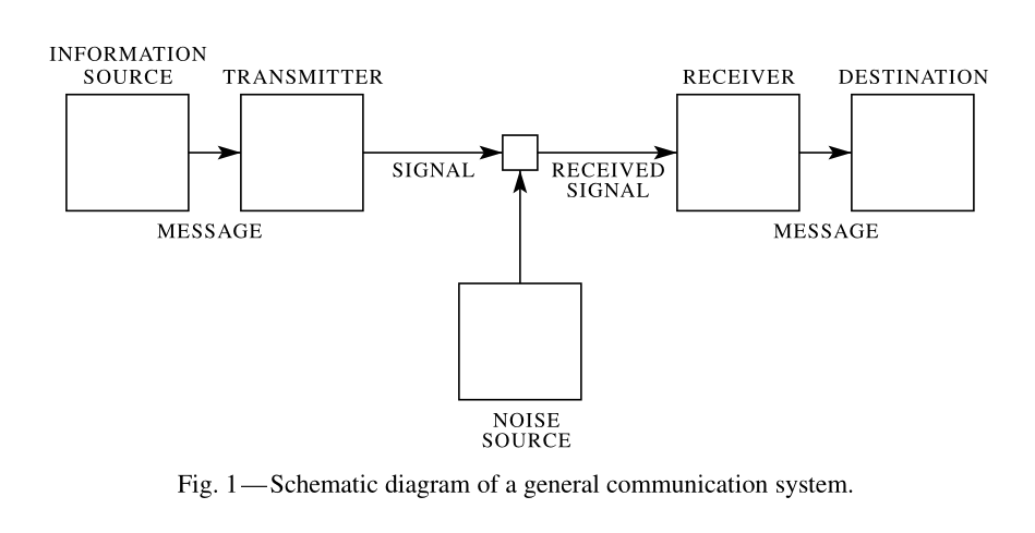
By a communication system we will mean a system of the type indicated schematically in Fig. 1. It consists of essentially five parts (Shannon, 1948, Introduction).


From A Mathematical Theory of Communication

An information source which produces a message or sequence of messages to be communicated to the receiving terminal (Shannon, 1948, Introduction). That message may be a sequence of letters, a function of time as in radio or telephony, a function of space and time as in television, several such functions as in multiplex or color television, or combinations of these. The source is where choice happens.

A transmitter which operates on the message in some way to produce a signal suitable for transmission over the channel (Shannon, 1948, Introduction). In telephony this operation consists merely of changing sound pressure into a proportional electrical current. In telegraphy we have an encoding operation which produces a sequence of dots, dashes and spaces on the channel corresponding to the message (Shannon, 1948, Introduction). In PCM the speech functions are sampled, compressed, quantized, encoded, and interleaved. Message and signal are not the same object. The transmitter is the map between them.

The channel is merely the medium used to transmit the signal from transmitter to receiver. It may be a pair of wires, a coaxial cable, a band of radio frequencies, a beam of light, etc. (Shannon, 1948, Introduction). The channel carries the signal, not the meaning.

The receiver ordinarily performs the inverse operation of that done by the transmitter, reconstructing the message from the signal (Shannon, 1948, Introduction). If the transmitter encodes, the receiver decodes.

The destination is the person (or thing) for whom the message is intended (Shannon, 1948, Introduction). The destination sits outside the engineering cut. What it does with the recovered message is not part of the five boxes.

This is a pipeline. Message, signal, and recovered message are three different objects. Confusing them is how people start talking about meaning when they mean bits.

We may roughly classify communication systems into three main categories: discrete, continuous and mixed (Shannon, 1948, Introduction). By a discrete system we will mean one in which both the message and the signal are a sequence of discrete symbols (Shannon, 1948, Introduction). Telegraphy is the typical case. A continuous system is one in which the message and signal are both treated as continuous functions, e.g., radio or television. A mixed system is one in which both discrete and continuous variables appear, e.g., PCM transmission of speech (Shannon, 1948, Introduction). PCM is mixed because the waveform is continuous and the transmitted symbols are discrete.

We first consider the discrete case. This case has applications not only in communication theory, but also in the theory of computing machines, the design of telephone exchanges and other fields. In addition the discrete case forms a foundation for the continuous and mixed cases (Shannon, 1948, Introduction). Computers and telegraphy are already discrete. Sampling will later turn analog into this same theory.

Discrete Noiseless Systems

The Discrete Noiseless Channel

Generally, a discrete channel will mean a system whereby a sequence of choices from a finite set of elementary symbols $S_1, \ldots, S_n$ can be transmitted from one point to another (Shannon, 1948, Section 1). Each of the symbols $S_i$ is assumed to have a certain duration in time $t_i$ seconds (not necessarily the same for different $S_i$, for example the dots and dashes in telegraphy) (Shannon, 1948, Section 1). It is not required that all possible sequences of the $S_i$ be capable of transmission on the system; certain sequences only may be allowed. These will be possible signals for the channel (Shannon, 1948, Section 1). Symbols can take different amounts of time, and not every concatenation is legal. Capacity has to count the legal ones.

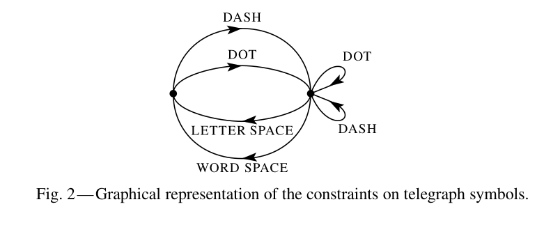
In telegraphy the symbols are a dot, a dash, a letter space, and a word space, with the restriction that two spaces cannot follow each other. The question we now consider is how one can measure the capacity of such a channel to transmit information (Shannon, 1948, Section 1). Capacity is a property of the allowed set of signals, not of the particular message you happen to send today.

In the teletype case where all symbols are of the same duration, and any sequence of the 32 symbols is allowed the answer is easy. Each symbol represents five bits of information. If the system transmits $n$ symbols per second it is natural to say that the channel has a capacity of $5n$ bits per second (Shannon, 1948, Section 1). This does not mean that the teletype channel will always be transmitting information at this rate - this is the maximum possible rate and whether or not the actual rate reaches this maximum depends on the source of information which feeds the channel (Shannon, 1948, Section 1). $5n$ is a ceiling. A source that repeats itself undershoots it. That gap is what encoding later tries to close.

In the general case Shannon defines capacity by

\[C = \lim_{T \to \infty} \frac{\log N(T)}{T}\]

where $N(T)$ is the number of allowed signals of duration $T$ (Shannon, 1948, Section 1). This means that the logarithm of the number of possible signals grows linearly with time, and $C$ is that slope, in bits per second.

If all sequences of symbols with durations $t_1, \ldots, t_n$ are allowed, $N(t)$ satisfies $N(t) = N(t-t_1) + \cdots + N(t-t_n)$. For large $t$, $N(t)$ behaves like $X_0^t$, where $X_0$ is the largest real root of

\[X^{-t_1} + X^{-t_2} + \cdots + X^{-t_n} = 1\]

and therefore $C = \log X_0$. In the telegraph example this gives $C \approx 0.539$ (Shannon, 1948, Section 1).

A very general type of restriction which may be placed on allowed sequences is a finite number of states: for each state only certain symbols from the set $S_1, \ldots, S_n$ can be transmitted and when one of these has been transmitted the state changes to a new state depending both on the old state and the particular symbol transmitted (Shannon, 1948, Section 1). Telegraphy has two states, according to whether the last symbol was a space. The conditions can be indicated in a linear graph as shown in Fig. 2 (Shannon, 1948, Section 1).


From A Mathematical Theory of Communication

Theorem 1: Let $b_{ij}^{(s)}$ be the duration of the $s$th symbol which is allowable in state $i$ and leads to state $j$. Then the channel capacity $C$ is equal to $\log W$ where $W$ is the largest real root of the determinant equation (Shannon, 1948, Section 1):

\[\left| \sum_s W^{-b_{ij}^{(s)}} - \delta_{ij} \right| = 0\]

The proof is a growth argument on the number of blocks ending in each state (Shannon, 1948, Appendix 1). This means channel capacity is the exponential growth rate of the set of allowed signals. Constraints change the allowed set. They do not change the fact that the set has a growth rate.

The Discrete Source of Information

We have seen that under very general conditions the logarithm of the number of possible signals in a discrete channel increases linearly with time (Shannon, 1948, Section 2). The next question is the source. The main point at issue is the effect of statistical knowledge about the source in reducing the required capacity of the channel, by the use of proper encoding of the information (Shannon, 1948, Section 2).

In telegraphy, for example, the messages to be transmitted consist of sequences of letters. These sequences, however, are not completely random. In general, they form sentences and have the statistical structure of, say, English. The letter E occurs more frequently than Q, the sequence TH more frequently than XP, etc. (Shannon, 1948, Section 2). The existence of this structure allows one to make a saving in time (or channel capacity) by properly encoding the message sequences into signal sequences. This is already done to a limited extent in telegraphy by using the shortest channel symbol, a dot, for the most common English letter E; while the infrequent letters, Q, X, Z are represented by longer sequences of dots and dashes (Shannon, 1948, Section 2).

We can think of a discrete source as generating the message, symbol by symbol. It will choose successive symbols according to certain probabilities depending, in general, on preceding choices as well as the particular symbols in question. A physical system, or a mathematical model of a system which produces such a sequence of symbols governed by a set of probabilities, is known as a stochastic process. We may consider a discrete source, therefore, to be represented by a stochastic process (Shannon, 1948, Section 2). A source is a probability law on strings. GPT training is the same claim at neural scale: estimate that law, then sample from it (Radford et al., 2019).

That includes natural languages, quantized continuous sources such as PCM speech, and abstract processes defined only by their probabilities. Shannon’s artificial examples make the ladder of dependence visible (Shannon, 1948, Section 2).

(A) Five letters A-E, each with probability $0.2$, chosen independently.

(B) The same letters with probabilities $0.4, 0.1, 0.2, 0.2, 0.1$, still independent.

(C) A more complicated structure is obtained if successive symbols are not chosen independently but their probabilities depend on preceding letters. In the simplest case of this type a choice depends only on the preceding letter and not on ones before that (Shannon, 1948, Section 2). The structure is a table of transition probabilities $p_i(j)$, or equivalently digram probabilities $p(i,j)$.

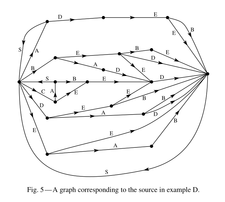
(D) A small vocabulary of sixteen “words” with given probabilities, chosen independently and separated by spaces.

These artificial languages are useful in constructing simple problems and examples to illustrate various possibilities. We can also approximate to a natural language by means of a series of simple artificial languages (Shannon, 1948, Section 2). A and B are independent letters. C is a Markoff letter source. D is a word source. English is approximated by climbing that ladder, which is the next section.

The Series of Approximations to English

To give a visual idea of how this series of processes approaches a language, typical sequences in the approximations to English have been constructed (Shannon, 1948, Section 3). In all cases we have assumed a 27-symbol “alphabet,” the 26 letters and a space (Shannon, 1948, Section 3).

Zero-order approximation (symbols independent and equiprobable). XFOML RXKHRJFFJUJ ZLPWCFWKCYJ FFJEYVKCQSGHYD QPAAMKBZAACIBZLHJQD.
First-order approximation (symbols independent but with frequencies of English text). OCRO HLI RGWR NMIELWIS EU LL NBNESEBYA TH EEI ALHENHTTPA OOBTTVA NAH BRL.
Second-order approximation (digram structure as in English). ON IE ANTSOUTINYS ARE T INCTORE ST BE S DEAMY ACHIN D ILONASIVE TUCOOWE AT TEASONARE FUSO TIZIN ANDY TOBE SEACE CTISBE.
Third-order approximation (trigram structure as in English). IN NO IST LAT WHEY CRATICT FROURE BIRS GROCID PONDENOME OF DEMONSTURES OF THE REPTAGIN IS REGOACTIONA OF CRE.
First-order word approximation. REPRESENTING AND SPEEDILY IS AN GOOD APT OR COME CAN DIFFERENT NATURAL HERE HE THE A IN CAME THE TO OF TO EXPERT GRAY COME TO FURNISHES THE LINE MESSAGE HAD BE THESE.
Second-order word approximation. THE HEAD AND IN FRONTAL ATTACK ON AN ENGLISH WRITER THAT THE CHARACTER OF THIS POINT IS THEREFORE ANOTHER METHOD FOR THE LETTERS THAT THE TIME OF WHO EVER TOLD THE PROBLEM FOR AN UNEXPECTED.

The resemblance to ordinary English text increases quite noticeably at each of the above steps (Shannon, 1948, Section 3). Note that these samples have reasonably good structure out to about twice the range that is taken into account in their construction (Shannon, 1948, Section 3). The ten-word stretch “attack on an English writer that the character of this” is not strained English. It appears then that a sufficiently complex stochastic process will give a satisfactory representation of a discrete source (Shannon, 1948, Section 3). More context makes the fake English look real. That is the same bet a language model makes: condition on more of the past, and the next token looks less random (Radford et al., 2018).

This is n-gram language modeling, written down in 1948 (Bengio et al., 2003). Letter frequencies, digrams, trigrams, then a jump to words because the labor of the next letter-order becomes enormous. A GPT-style transformer is what happens when that labor is no longer the bottleneck: instead of stopping at trigrams, the model conditions on thousands of tokens and is trained by driving cross-entropy toward the entropy of the source (Vaswani et al., 2017; Radford et al., 2018). The first two samples were constructed by the use of a book of random numbers in conjunction with a table of letter frequencies (Shannon, 1948, Section 3). For the later samples Shannon opened a book, found the current letter, and took the next one. It would be interesting if further approximations could be constructed, but the labor involved becomes enormous at the next stage (Shannon, 1948, Section 3). He stopped at trigrams because the tables explode. Transformers buy that extra context without storing an n-gram table.

Graphical Representation of a Markoff Process

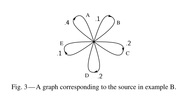
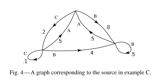
Stochastic processes of the type described above are known mathematically as discrete Markoff processes (Shannon, 1948, Section 4). There exist a finite number of possible “states” of a system; $S_1, S_2, \ldots, S_n$. In addition there is a set of transition probabilities; $p_i(j)$ the probability that if the system is in state $S_i$ it will next go to state $S_j$. To make this Markoff process into an information source we need only assume that a letter is produced for each transition from one state to another. The states will correspond to the “residue of influence” from preceding letters (Shannon, 1948, Section 4). The state is just enough past to fix the next-letter distribution. You do not need the whole history, only the residue that still affects the next choice.


From A Mathematical Theory of Communication


From A Mathematical Theory of Communication

Fig. 3 is for the example B in Section 2, a single state with five independent letters. Fig. 4 corresponds to the example C (Shannon, 1948, Section 4), one state per letter, because the next letter depends on the current one. A closed series of lines with arrows in the same orientation is a circuit. The structure of those circuits is what decides whether the source has a single long-run behaviour or several.

Ergodic and Mixed Sources

Not every Markoff source has a single entropy that you can treat as the rate of the source. Shannon isolates the case that does. Fig. 5 is a graph for the case of word structure in example D. Here S corresponds to the “space” symbol (Shannon, 1948, Section 4). The graph should not consist of two isolated parts A and B such that it is impossible to go from A to B. A closed series of lines in the graph with all arrows pointing in the same orientation should not have a greatest common divisor of lengths greater than one (Shannon, 1948, Section 5). When those conditions hold, the source is ergodic.


From A Mathematical Theory of Communication

In the ergodic case it can be shown that with any starting conditions the probabilities $P_j(N)$ of being in state $j$ after $N$ symbols, approach the equilibrium values as $N \to \infty$ (Shannon, 1948, Section 5). This means long typical sequences all look like the source. A mixed source is a combination of ergodic components. Which component you are in may be a permanent accident of the starting state. Entropy is a single number only when the source is ergodic.

Choice, Uncertainty and Entropy

We have represented a discrete information source as a Markoff process. Can we define a quantity which will measure, in some sense, how much information is “produced” by such a process, or better, at what rate information is produced? (Shannon, 1948, Section 6).

Suppose we have a set of possible events whose probabilities of occurrence are $p_1, p_2, \ldots, p_n$. These probabilities are known but that is all we know concerning which event will occur. Can we find a measure of how much “choice” is involved in the selection of the event or of how uncertain we are of the outcome? (Shannon, 1948, Section 6). If there is such a measure $H(p_1, \ldots, p_n)$, Shannon requires three properties. The properties are a specification, not a derivation. They say what “amount of choice” is allowed to mean.

$H$ should be continuous in the $p_i$ (Shannon, 1948, Section 6). A tiny change in probability should not jump the measure.
If all the $p_i$ are equal, $p_i = 1/n$, then $H$ should be a monotonic increasing function of $n$. With equally likely events there is more choice, or uncertainty, when there are more possible events (Shannon, 1948, Section 6). Ten equally likely outcomes should be more uncertain than two.
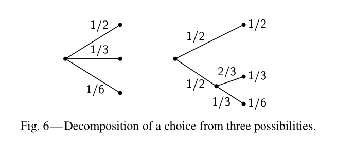
If a choice be broken down into two successive choices, the original $H$ should be the weighted sum of the individual values of $H$. The meaning of this is illustrated in Fig. 6 (Shannon, 1948, Section 6). Entropy of a two-stage choice is the first choice plus the weighted second choice. Surprise has to add that way, or the measure is not a rate.


From A Mathematical Theory of Communication

The grouping axiom is the important one. Three outcomes with probabilities $1/2$, $1/3$, $1/6$ can be chosen directly, or by first choosing between two groups of probability $1/2$ each and then, half the time, making a second choice with probabilities $2/3$ and $1/3$. We require, in this special case, that

\[H\left(\tfrac{1}{2},\tfrac{1}{3},\tfrac{1}{6}\right) = H\left(\tfrac{1}{2},\tfrac{1}{2}\right) + \tfrac{1}{2}\, H\left(\tfrac{2}{3},\tfrac{1}{3}\right)\]

(Shannon, 1948, Section 6).

Theorem 2: The only $H$ satisfying the three above assumptions is of the form

\[H = -K \sum_{i=1}^{n} p_i \log p_i\]

where $K$ is a positive constant (Shannon, 1948, Section 6, Appendix 2). This theorem, and the assumptions required for its proof, are in no way necessary for the present theory. It is given chiefly to lend a certain plausibility to some of our later definitions. The real justification of these definitions, however, will reside in their implications (Shannon, 1948, Section 6). The formula is not true because the axioms are pretty. It is true because the coding theorems later say you can compress to this $H$ and not below.

Quantities of the form $H = -\sum p_i \log p_i$ play a central role in information theory as measures of information, choice and uncertainty. The form of $H$ will be recognized as that of entropy as defined in certain formulations of statistical mechanics where $p_i$ is the probability of a system being in cell $i$ of its phase space. $H$ is then, for example, the $H$ in Boltzmann’s famous H theorem. We shall call $H = -\sum p_i \log p_i$ the entropy of the set of probabilities $p_1, \ldots, p_n$ (Shannon, 1948, Section 6). The name is borrowed from physics. The operational meaning here is bits of choice, not temperature.

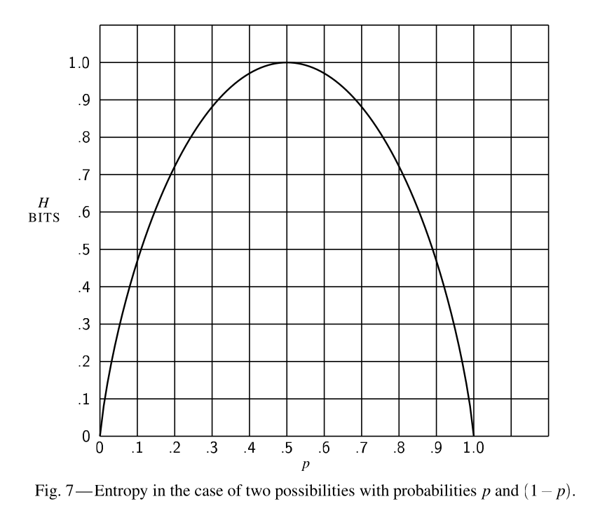
The binary case $H = -(p \log p + q \log q)$ with $q = 1-p$ is plotted in Fig. 7 as a function of $p$ (Shannon, 1948, Section 6).


From A Mathematical Theory of Communication

The quantity $H$ has a number of interesting properties which further substantiate it as a reasonable measure of choice or information (Shannon, 1948, Section 6).

$H = 0$ if and only if all the $p_i$ but one are zero, this one having the value unity. Thus only when we are certain of the outcome does $H$ vanish. Otherwise $H$ is positive (Shannon, 1948, Section 6).
For a given $n$, $H$ is a maximum and equal to $\log n$ when all the $p_i$ are equal (i.e., $1/n$). This is also intuitively the most uncertain situation (Shannon, 1948, Section 6).
The uncertainty of a joint event is less than or equal to the sum of the individual uncertainties, $H(x,y) \leq H(x) + H(y)$, with equality only if the events are independent (Shannon, 1948, Section 6).
Any change toward equalization of the probabilities $p_1, p_2, \ldots, p_n$ increases $H$ (Shannon, 1948, Section 6).
The conditional entropy $H_x(y)$ is the average uncertainty in $y$ when $x$ is known. Then $H(x,y) = H(x) + H_x(y)$. The uncertainty (or entropy) of the joint event $x,y$ is the uncertainty of $x$ plus the uncertainty of $y$ when $x$ is known (Shannon, 1948, Section 6).
The uncertainty of $y$ is never increased by knowledge of $x$. It will be decreased unless $x$ and $y$ are independent events, in which case it is not changed (Shannon, 1948, Section 6).

Certainty is 0. Uniformity is the maximum. Extra knowledge cannot increase $H$. That last property is why $H(x) - H_y(x)$ can be a rate of information: it is the surprise that $y$ removes. Shannon does not yet call it mutual information. He will use it as the rate of transmission the moment noise appears. A fair coin is 1 bit. A rigged coin that always comes up heads is 0 bits. Colah’s diagrams are a later visual restatement of the same $H$ (Colah, 2015).

The Entropy of an Information Source

Consider a discrete source of the finite state type considered above. For each possible state $i$ there will be a set of probabilities $p_i(j)$ of producing the various possible symbols $j$. Thus there is an entropy $H_i$ for each state. The entropy of the source will be defined as the average of these $H_i$ weighted in accordance with the probability of occurrence of the states in question (Shannon, 1948, Section 7):

\[H = \sum_i P_i H_i = -\sum_{i,j} P_i p_i(j) \log p_i(j)\]

This is the entropy of the source per symbol of text (Shannon, 1948, Section 7). If the process runs at a definite rate there is also an entropy per second $H' = mH$. $H$ or $H'$ measures the amount of information generated by the source per symbol or per second. If the logarithmic base is 2, they will represent bits per symbol or per second (Shannon, 1948, Section 7). Source rate is an average over states, not the surprise of one letter. A rare letter in a rare state still only contributes according to how often that state is occupied.

For a long independent message of $N$ symbols, it will contain with high probability about $p_1 N$ occurrences of the first symbol, $p_2 N$ occurrences of the second, etc. (Shannon, 1948, Section 7). Then $\log p \approx -NH$, or

\[H \approx \frac{\log 1/p}{N}\]

$H$ is thus approximately the logarithm of the reciprocal probability of a typical long sequence divided by the number of symbols in the sequence. The same result holds for any source (Shannon, 1948, Section 7).

Theorem 3: Given any $\varepsilon > 0$ and $\delta > 0$, we can find an $N_0$ such that the sequences of any length $N \geq N_0$ fall into two classes: 1. A set whose total probability is less than $\varepsilon$. 2. The remainder, all of whose members have probabilities satisfying

\[\left| \frac{\log p^{-1}}{N} - H \right| < \delta\]

(Shannon, 1948, Section 7). In other words we are almost certain to have $\log p^{-1}/N$ very close to $H$ when $N$ is large (Shannon, 1948, Section 7). This means almost every long sequence has probability about $2^{-NH}$. The rare sequences can be ignored.

Theorem 4:

\[\lim_{N \to \infty} \frac{\log n(q)}{N} = H\]

when $q$ does not equal 0 or 1 (Shannon, 1948, Section 7). Here $n(q)$ is how many sequences, starting from the most probable, you must take to accumulate total probability $q$. We may interpret $\log n(q)$ as the number of bits required to specify the sequence when we consider only the high-probability set (Shannon, 1948, Section 7). This means the typical set has about $2^{NH}$ members. Cover and Thomas later call this the asymptotic equipartition property (Cover and Thomas, 2006).

Theorems 5 and 6 identify the same $H$ as a limit of block entropies $G_N$ and of conditional entropies given a growing past (Shannon, 1948, Section 7, Appendix 3). Those two facts, that typical sequences all have probability $2^{-NH}$ and that there are about $2^{NH}$ of them, are the engine of the coding theorems. The conditional-entropy limit is also the training objective of a GPT-style model: the loss on each token is the surprise of that token given the past (Radford et al., 2018).

Encoding and Decoding as Finite State Transducers

Encoding is a finite-state transducer: an input symbol, together with the current state, produces an output block and a next state (Shannon, 1948, Section 8). If there exists a second transducer which operates on the output of the first and recovers the original input, the first transducer will be called non-singular and the second will be called its inverse (Shannon, 1948, Section 8).

Theorem 7: The output of a finite state transducer driven by a finite state statistical source is a finite state statistical source, with entropy (per unit time) less than or equal to that of the input. If the transducer is non-singular they are equal (Shannon, 1948, Section 8).

This means you cannot create information by encoding. You can throw some of it away. A reversible encoder leaves the entropy rate unchanged, which is why a noiseless channel’s input entropy cannot exceed its capacity.

Theorem 8: Let the system of constraints considered as a channel have a capacity $C = \log W$. There is an assignment of transition probabilities on the constraint graph that maximizes the entropy of the resulting source, then $H$ is maximized and equal to $C$ (Shannon, 1948, Section 8). By proper assignment of the transition probabilities the entropy of symbols on a channel can be maximized at the channel capacity (Shannon, 1948, Section 8). The most you can feed a constrained channel is $C$, and you get there by matching the source’s transitions to the assignment that saturates the allowed graph. Encoding is that matching.

The Fundamental Theorem for a Noiseless Channel

We will now justify our interpretation of $H$ as the rate of generating information by proving that $H$ determines the channel capacity required with most efficient coding (Shannon, 1948, Section 9). Until this theorem, $H$ was a plausible formula. After it, $H$ is the number of bits you actually need.

Theorem 9: Let a source have entropy $H$ (bits per symbol) and a channel have a capacity $C$ (bits per second). Then it is possible to encode the output of the source in such a way as to transmit at the average rate $C/H - \varepsilon$ symbols per second over the channel where $\varepsilon$ is arbitrarily small. It is not possible to transmit at an average rate greater than $C/H$ (Shannon, 1948, Section 9). This is the source-coding theorem. Compress to $H$ bits per symbol. You cannot do better. With delay you can come arbitrarily close.

The converse is immediate from Theorem 7. The encoder must be non-singular, so the entropy per second of the channel input equals that of the source, and that entropy cannot exceed $C$.

The direct half is proved twice. The first proof uses the typical set. Sequences of length $N$ split into a high-probability group with fewer than $2^{(H+\eta)N}$ members and a leftover of vanishing total probability. For large $T$ the channel has more than $2^{(C-\theta)T}$ signals. Choosing $T$ a little larger than $NH/C$ leaves enough channel sequences for a one-to-one map of the typical set (Shannon, 1948, Section 9).

The second proof is the construction found independently by R. M. Fano. Arrange the messages of length $N$ in decreasing probability. Let $P_s$ be the cumulative probability strictly before $p_s$. Encode message $s$ as the binary expansion of $P_s$, taken to $m_s$ places, where

\[\log_2 \frac{1}{p_s} \leq m_s < 1 + \log_2 \frac{1}{p_s}\]

Thus the messages of high probability are represented by short codes and those of low probability by long codes (Shannon, 1948, Section 9). The average number of binary digits per original symbol, $H'$, satisfies $G_N \leq H' < G_N + 1/N$, and $G_N \to H$. We see from this that the inefficiency in coding, when only a finite delay of $N$ symbols is used, need not be greater than $1/N$ plus the difference between the true entropy $H$ and the entropy $G_N$ calculated for sequences of length $N$ (Shannon, 1948, Section 9). The fractional excess time over the ideal is less than

\[\frac{G_N}{H} + \frac{1}{HN} - 1\]

This method of encoding is substantially the same as one found independently by R. M. Fano (Shannon, 1948, Section 9; Fano, 1949). His method splits the messages into two groups of as nearly equal probability as possible and assigns 0 or 1, then repeats. Huffman later gave the optimal prefix code for the same problem (Huffman, 1952).

Matching the Source to the Channel

In order to obtain the maximum power transfer from a generator to a load, a transformer must in general be introduced so that the generator as seen from the load has the load resistance. The situation here is roughly analogous. The transducer which does the encoding should match the source to the channel in a statistical sense (Shannon, 1948, Section 10). The content of Theorem 9 is that, although an exact match is not in general possible, we can approximate it as closely as desired. The ratio of the actual rate of transmission to the capacity $C$ may be called the efficiency of the coding system (Shannon, 1948, Section 10). Encoding is impedance matching. The source, seen through the encoder, should look like the source that saturates the channel.

In general, ideal or nearly ideal encoding requires a long delay in the transmitter and receiver. In the noiseless case which we have been considering, the main function of this delay is to allow reasonably good matching of probabilities to corresponding lengths of sequences (Shannon, 1948, Section 10). With a good code the logarithm of the reciprocal probability of a long message must be proportional to the duration of the corresponding signal (Shannon, 1948, Section 10). Delay is how you wait for a typical block. Short, rare messages get long codes. Common blocks get short ones. That matching is bad until $N$ is large.

If a source can produce only one particular message its entropy is zero, and no channel is required. For example, a computing machine set up to calculate the successive digits of $\pi$ produces a definite sequence with no chance element. No channel is required to “transmit” this to another point. One could construct a second machine to compute the same sequence at the point. However, this may be impractical. In such a case we can choose to ignore some or all of the statistical knowledge we have of the source (Shannon, 1948, Section 10). Treating the digits of $\pi$ as random decimal digits retains only that they come from $\{0, \ldots, 9\}$. In the case of English one might wish to use the statistical saving possible due to letter frequencies, but nothing else. The maximum entropy source is then the first approximation to English and its entropy determines the required channel capacity (Shannon, 1948, Section 10).

As a simple example of some of these results consider a source which produces a sequence of letters chosen from among A, B, C, D with probabilities $1/2$, $1/4$, $1/8$, $1/8$, successive symbols being chosen independently (Shannon, 1948, Section 10). Then

\[H = -\left(\tfrac{1}{2}\log\tfrac{1}{2} + \tfrac{1}{4}\log\tfrac{1}{4} + \tfrac{2}{8}\log\tfrac{1}{8}\right) = \tfrac{7}{4}\ \text{bits per symbol}\]

Thus we can approximate a coding system to encode messages from this source into binary digits with an average of $7/4$ binary digit per symbol. In this case we can actually achieve the limiting value by the following code (obtained by the method of the second proof of Theorem 9) (Shannon, 1948, Section 10):

Symbol	Code
A	0
B	10
C	110
D	111

The average length is $\tfrac{1}{2}\cdot 1 + \tfrac{1}{4}\cdot 2 + \tfrac{2}{8}\cdot 3 = 7/4$. The maximum possible entropy for the original set is $\log 4 = 2$, occurring when A, B, C, D have probabilities $1/4, 1/4, 1/4, 1/4$. Hence the relative entropy is $7/8$ (Shannon, 1948, Section 10). The source has slack of $1/8$ because the letters are not equiprobable. The code spends that slack: A is a single 0, D takes three bits. Mapping pairs of bits back onto A, B, C, D compresses the original message by that factor.

The Discrete Channel with Noise

Distortion Versus Noise

We now consider the case where the signal is perturbed by noise during transmission or at one or the other of the terminals. This means that the received signal is not necessarily the same as that sent out by the transmitter (Shannon, 1948, Section 11). Two cases may be distinguished. If a particular transmitted signal always produces the same received signal, i.e., the received signal is a definite function of the transmitted signal, then the effect may be called distortion. If this function has an inverse - no two transmitted signals producing the same received signal - distortion may be corrected, at least in principle, by merely performing the inverse functional operation on the received signal (Shannon, 1948, Section 11). Distortion is a fixed map. If it is invertible, you undo it. You do not need statistics for that.

The case of interest here is that in which the signal does not always undergo the same change in transmission (Shannon, 1948, Section 11). Then $E = f(S, N)$, with $N$ a chance variable. When successive symbols are perturbed independently, the channel is a table of transition probabilities $p_i(j)$. Noise is random. The same sent symbol can come out two different ways, so there is no inverse map. You need probabilities.

If a noisy channel is fed by a source there are two statistical processes at work: the source and the noise. Thus there are a number of entropies that can be calculated (Shannon, 1948, Section 11). $H(x)$ of the input, $H(y)$ of the output, $H(x,y)$ of the pair, and the two conditional entropies $H_x(y)$ and $H_y(x)$. Among these quantities we have the relations

\[H(x,y) = H(x) + H_x(y) = H(y) + H_y(x)\]

(Shannon, 1948, Section 11). In the noiseless case, $H(y) = H(x)$ and $H_y(x) = 0$.

Equivocation and Channel Capacity

If the channel is noisy it is not in general possible to reconstruct the original message or the transmitted signal with certainty by any operation on the received signal $E$. There are, however, ways of transmitting the information which are optimal in combating noise (Shannon, 1948, Section 12).

Suppose there are two possible symbols 0 and 1, and we are transmitting at a rate of 1000 symbols per second with probabilities $p_0 = p_1 = 1/2$. Thus our source is producing information at the rate of 1000 bits per second. During transmission the noise introduces errors so that, on the average, 1 in 100 is received incorrectly (Shannon, 1948, Section 12). What is the rate of transmission of information? Certainly less than 1000 bits per second since about 1% of the received symbols are incorrect. Our first impulse might be to say the rate is 990 bits per second, merely subtracting the expected number of errors. This is not satisfactory since it fails to take into account the recipient’s lack of knowledge of where the errors occur (Shannon, 1948, Section 12).

We may carry it to an extreme case and suppose the noise so great that the received symbols are entirely independent of the transmitted symbols (Shannon, 1948, Section 12). Then about half of the received symbols are correct due to chance alone, and we would be giving the system credit for transmitting 500 bits per second while actually no information is being transmitted at all. Equally “good” transmission would be obtained by dispensing with the channel entirely and flipping a coin at the receiving point (Shannon, 1948, Section 12). Subtracting the error rate credits chance. If half the bits match by luck, you have not received 500 bits of information. You have received a coin flip.

Evidently the proper correction to apply to the amount of information transmitted is the amount of this information which is missing in the received signal, or alternatively the uncertainty when we have received a signal of what was actually sent (Shannon, 1948, Section 12). Following this idea the rate of actual transmission, $R$, would be obtained by subtracting from the rate of production (i.e., the entropy of the source) the average rate of conditional entropy (Shannon, 1948, Section 12):

\[R = H(x) - H_y(x)\]

The conditional entropy $H_y(x)$ will, for convenience, be called the equivocation. It measures the average ambiguity of the received signal (Shannon, 1948, Section 12). Equivocation is not the error rate. It is leftover uncertainty about what was sent, given what arrived. That is why 1% flips cost 81 bits per second, not 10.

In the 1% error example, if a 0 is received the a posteriori probability that a 0 was transmitted is .99, and that a 1 was transmitted is .01 (Shannon, 1948, Section 12). Then $H_y(x) \approx 0.081$ bits per symbol, or 81 bits per second, and we may say that the system is transmitting at a rate $1000 - 81 = 919$ bits per second (Shannon, 1948, Section 12). In the coin-flip extreme, $H_y(x) = 1$ bit per symbol and $R = 0$.

The same $R$ has two other writings:

\[R = H(x) - H_y(x) = H(y) - H_x(y) = H(x) + H(y) - H(x,y)\]

The first defining expression has already been interpreted as the amount of information sent less the uncertainty of what was sent. The second measures the amount received less the part of this which is due to noise. The third is the sum of the two amounts less the joint entropy and therefore in a sense is the number of bits per second common to the two (Shannon, 1948, Section 12). All three are the same overlap. $R$ is the uncertainty that input and output share. Equivocation is the part of the input that the output does not pin down.

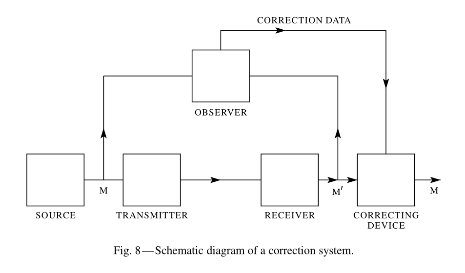
The situation is indicated schematically in Fig. 8 (Shannon, 1948, Section 12).

Theorem 10: If the correction channel has a capacity equal to $H_y(x)$ it is possible to so encode the correction data as to send it over this channel and correct all but an arbitrarily small fraction of the errors. This is not possible if the channel capacity is less than $H_y(x)$ (Shannon, 1948, Section 12).


From A Mathematical Theory of Communication

Roughly then, $H_y(x)$ is the amount of additional information that must be supplied per second at the receiving point to correct the received message (Shannon, 1948, Section 12). A side channel of capacity $H_y(x)$ is necessary and sufficient to clean the output. Less than that, some errors stay. That is the operational meaning of equivocation.

The capacity $C$ of a noisy channel should be the maximum possible rate of transmission, i.e., the rate when the source is properly matched to the channel. We therefore define the channel capacity by

\[C = \max \big( H(x) - H_y(x) \big)\]

where the maximum is with respect to all possible information sources used as input to the channel (Shannon, 1948, Section 12). If the channel is noiseless, $H_y(x) = 0$. The definition is then equivalent to that already given for a noiseless channel (Shannon, 1948, Section 12). Capacity is not the rate of whatever source you happen to plug in. It is the best matched source. A poorly chosen input distribution leaves rate on the table.

The Fundamental Theorem for a Discrete Channel with Noise

It may seem surprising that we should define a definite capacity $C$ for a noisy channel since we can never send certain information in such a case. It is clear, however, that by sending the information in a redundant form the probability of errors can be reduced. For example, by repeating the message many times and by a statistical study of the different received versions of the message the probability of errors could be made very small. One would expect, however, that to make this probability of errors approach zero, the redundancy of the encoding must increase indefinitely, and the rate of transmission therefore approach zero. This is by no means true (Shannon, 1948, Section 13). The naive picture is: more reliability, more repetition, rate goes to zero. Shannon’s point is that this tradeoff has a corner. There is a rate $C$ at which you can buy arbitrarily high reliability without sending the rate to zero.

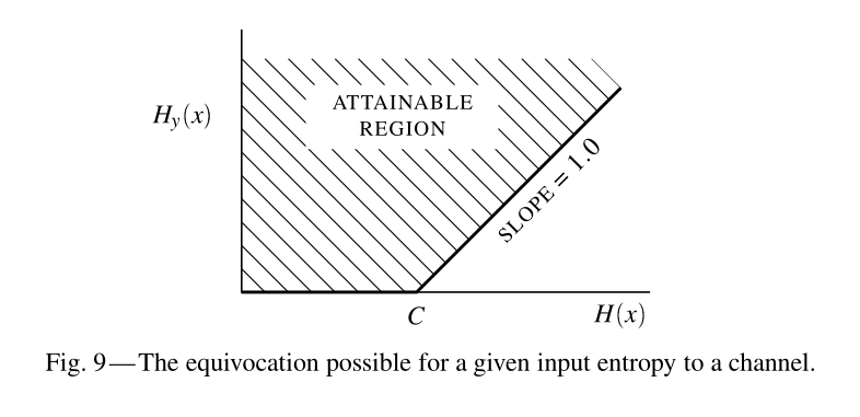
If it were, there would not be a very well defined capacity, but only a capacity for a given frequency of errors, or a given equivocation; the capacity going down as the error requirements are made more stringent. Actually the capacity $C$ defined above has a very definite significance. It is possible to send information at the rate $C$ through the channel with as small a frequency of errors or equivocation as desired by proper encoding. This statement is not true for any rate greater than $C$ (Shannon, 1948, Section 13). If an attempt is made to transmit at a higher rate than $C$, say $C + R_1$, then there will necessarily be an equivocation equal to or greater than the excess $R_1$. Nature takes payment by requiring just that much uncertainty, so that we are not actually getting any more than $C$ through correctly (Shannon, 1948, Section 13). Repeating a message can drive error down, but only by killing rate. Below $C$ you can have both low error and a positive rate. Above $C$ the extra rate is not information. It is leftover uncertainty. The situation is indicated in Fig. 9 (Shannon, 1948, Section 13). The rate of information into the channel is plotted horizontally and the equivocation vertically.


From A Mathematical Theory of Communication

Theorem 11: Let a discrete channel have the capacity $C$ and a discrete source the entropy per second $H$. If $H \leq C$ there exists a coding system such that the output of the source can be transmitted over the channel with an arbitrarily small frequency of errors (or an arbitrarily small equivocation). If $H > C$ it is possible to encode the source so that the equivocation is less than $H - C + \varepsilon$ where $\varepsilon$ is arbitrarily small. There is no method of encoding which gives an equivocation less than $H - C$ (Shannon, 1948, Section 13). This is the noisy-channel coding theorem. Rate below $C$, error can be driven to zero. Rate above $C$, you pay the excess as equivocation, always.

The method of proving the first part of this theorem is not by exhibiting a coding method having the desired properties, but by showing that such a code must exist in a certain group of codes (Shannon, 1948, Section 13). Average the error frequency over the group. If the average is less than $\varepsilon$, some member is less than $\varepsilon$. That is existence via random coding, not a construction you can implement tomorrow. Hamming’s later example is the rare case where a structured code meets $C$ on a hand-built noise model.

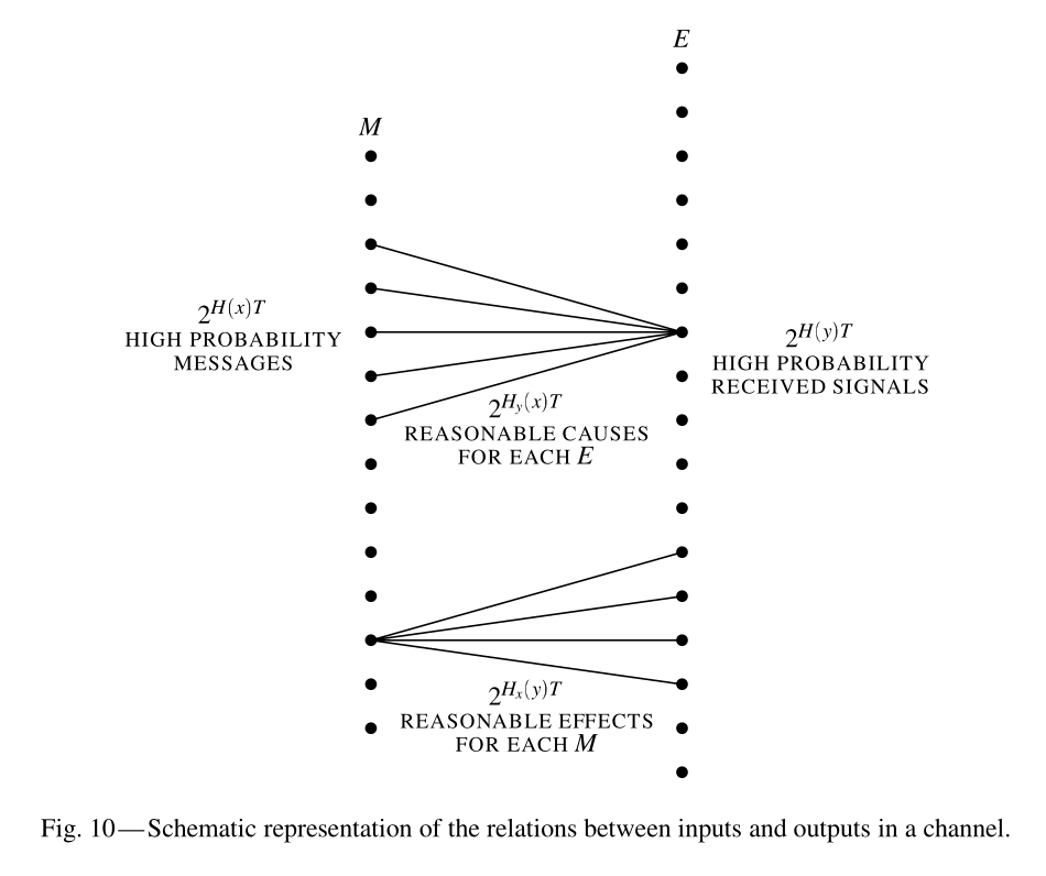
For long duration $T$, the transmitted sequences fall into two classes, a high probability group with about $2^{T H(x)}$ members and the remaining sequences of small total probability. Similarly the received sequences have a high probability set of about $2^{T H(y)}$ members. Each high probability output could be produced by about $2^{T H_y(x)}$ inputs (Shannon, 1948, Section 13). The situation is summarized in Fig. 10 where the input sequences are points on the left and output sequences points on the right (Shannon, 1948, Section 13). The fan of cross lines represents the range of possible causes for a typical output.


From A Mathematical Theory of Communication

Associate the typical messages of a source of rate $R < C$ at random with a selection of channel inputs. The fans of possible causes overlap little when $R$ is below $C$, so a decoder that picks the most probable cause in the codebook is rarely wrong. This means noise does not set a floor on error. It sets a ceiling on rate.

The demonstration of Theorem 11, while not a pure existence proof, has some of the deficiencies of such a proof (Shannon, 1948, Section 14). A random code of large block length works. Finding a structured code with the same performance is a different problem.

How Many Signals Can You Distinguish

Theorem 12:

\[\lim_{T \to \infty} \frac{\log N(T, q)}{T} = C\]

where $N(T, q)$ is the maximum number of signals of duration $T$ that can be chosen so that the probability of an incorrect interpretation is at most $q$, provided $q$ does not equal 0 or 1 (Shannon, 1948, Section 14). In other words, no matter how we set our limits of reliability, we can distinguish reliably in time $T$ enough messages to correspond to about $CT$ bits, when $T$ is sufficiently large. Theorem 12 can be compared with the definition of the capacity of a noiseless channel given in Section 1 (Shannon, 1948, Section 14). Noisy capacity is the same growth-rate idea as Section 1, counted over distinguishable signals rather than all allowed signals. Reliability $q$ drops out of the limit as long as it is not 0 or 1.

Examples of Discrete Channels and Their Capacity

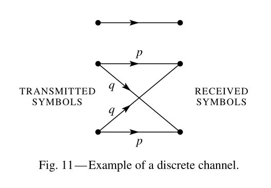
A simple example of a discrete channel is indicated in Fig. 11. There are three possible symbols. The first is never affected by noise. The second and third each have probability $p$ of coming through undisturbed, and $q$ of being changed into the other of the pair (Shannon, 1948, Section 15).


From A Mathematical Theory of Communication

Let $\gamma = -[p\log_2 p + q\log_2 q]$, and let $P$ and $Q$ be the probabilities of using the first symbol and one of the other two, with $P + 2Q = 1$. Maximizing $H(x) - H_y(x)$ gives

\[C = \log_2(2 + 2^{\gamma}) - \gamma\]

Note how this checks the obvious values in the cases $p = 1$ and $p = 1/2$ (Shannon, 1948, Section 15). When $p = 1$ the channel is noiseless and $C = \log_2 3$. When $p = 1/2$, the second and third symbols cannot be distinguished at all and act together like one symbol, so $C = 1$ bit (Shannon, 1948, Section 15). For intermediate values of $p$ the channel capacity will lie between $\log 2$ and $\log 3$. The first symbol is used somewhat more frequently than the other two because of its freedom from noise (Shannon, 1948, Section 15). Use the clean symbol more often. When the noisy pair is fully confused, it collapses to one symbol, and capacity drops from $\log 3$ to 1 bit. The formula interpolates between those two obvious designs.

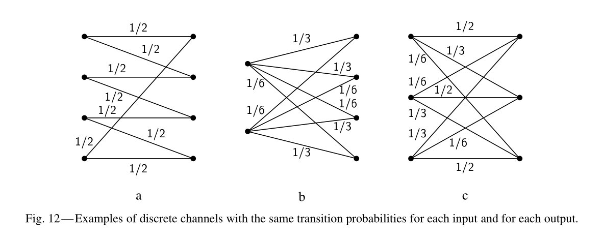
When every input symbol has the same fan of transition probabilities, and every output symbol the same incoming fan, $H_x(y)$ is independent of the distribution of probabilities on the input symbols (Shannon, 1948, Section 16). Capacity collapses to

\[C = \log m + \sum p_i \log p_i\]

where $m$ is the number of output symbols. Examples are shown in Fig. 12 (Shannon, 1948, Section 16).


From A Mathematical Theory of Communication

In Fig. 12a it would be $C = \log 4 - \log 2 = \log 2$, achieved by using only the 1st and 3d symbols (Shannon, 1948, Section 16). If symbols fall into groups that noise never confuses, the total probability $P_n$ of all symbols in the $n$th group should be $P_n = 2^{C_n}/\sum 2^{C_n}$, and the channel capacity is $C = \log \sum 2^{C_n}$ (Shannon, 1948, Section 16). Independent clean groups combine like parallel channels. You put more probability on the group with larger $C_n$, exponentially, the same way you would split power across parallel pipes.

An Example of Efficient Coding

The following example, although somewhat unrealistic, is a case in which exact matching to a noisy channel is possible. There are two channel symbols, 0 and 1, and the noise affects them in blocks of seven symbols. A block of seven is either transmitted without error, or exactly one symbol of the seven is incorrect. These eight possibilities are equally likely (Shannon, 1948, Section 17). The capacity is

\[C = \max\big(H(y) - H_x(y)\big) = 1 - \frac{\log_2 8}{7} = \tfrac{4}{7}\ \text{bits per symbol}\]

An efficient code, allowing complete correction of errors and transmitting at the rate $C$, is the following (found by a method due to R. Hamming) (Shannon, 1948, Section 17; Hamming, 1950). In a block $X_1, \ldots, X_7$, the positions $X_3, X_5, X_6, X_7$ are message bits. The other three are parity bits chosen to make three even-parity checks. When a block of seven is received the three checks are calculated and if even called zero, if odd called one. The binary number then gives the subscript of the $X_i$ that is incorrect (if 0 there was no error) (Shannon, 1948, Section 17).

This is the Hamming (7, 4) code, sitting in Shannon’s paper as a worked example of what Theorem 11 promised: a structured encoding that meets capacity for a very particular noise model.

Mathematical Preliminaries

Communication theory is properly concerned, as has been emphasized by Wiener, not with operations on particular functions, but with operations on ensembles of functions. A communication system is designed not for a particular speech function and still less for a sine wave, but for the ensemble of speech functions (Shannon, 1948, Section 18; Wiener, 1949). You design for the set of possible waveforms, not for one recording. A telephone that only worked for one sentence would not be a communication system.

Band Limited Ensembles

If a function of time $f(t)$ is limited to the band from 0 to $W$ cycles per second it is completely determined by giving its ordinates at a series of discrete points spaced $1/(2W)$ seconds apart (Shannon, 1948, Section 19).

Theorem 13: Let $f(t)$ contain no frequencies over $W$. Then

\[f(t) = \sum_{n=-\infty}^{\infty} X_n \frac{\sin \pi (2Wt - n)}{\pi (2Wt - n)}, \qquad X_n = f\left(\frac{n}{2W}\right)\]

(Shannon, 1948, Section 19). A function can be considered to be substantially limited to a time $T$ if all the ordinates $X_n$ outside this interval of time are zero. In this case all but $2TW$ of the coordinates will be zero. Thus functions limited to a band $W$ and duration $T$ correspond to points in a space of $2TW$ dimensions (Shannon, 1948, Section 19). One second of band-$W$ audio is a vector of $2W$ numbers. Sampling turns analog into the discrete theory (Nyquist, 1928; Shannon, 1949). That is why PCM can replace a waveform with a sequence of numbers, and why the first half of the paper is a foundation rather than a special case.

Entropy of a Continuous Distribution

The entropy of a discrete set of probabilities $p_1, \ldots, p_n$ has been defined as $H = -\sum p_i \log p_i$. In an analogous manner we define the entropy of a continuous distribution with the density distribution function $p(x)$ by (Shannon, 1948, Section 20):

\[H = -\int_{-\infty}^{\infty} p(x) \log p(x)\, dx\]

The entropies of continuous distributions have most (but not all) of the properties of the discrete case (Shannon, 1948, Section 20). Entropy is maximized, for a variable confined to a volume $v$, by the uniform distribution. $H(x,y) \leq H(x)+H(y)$ with equality for independence. For fixed average power, the maximum-entropy distribution is Gaussian. For a variable confined to a half-line with fixed mean $a$, the maximum is the exponential.

There is one important difference between the continuous and discrete entropies. In the discrete case the entropy measures in an absolute way the randomness of the chance variable. In the continuous case the measurement is relative to the coordinate system. If we change coordinates the entropy will in general change (Shannon, 1948, Section 20). In spite of this dependence on the coordinate system the entropy concept is as important in the continuous case as the discrete case. This is due to the fact that the derived concepts of information rate and channel capacity depend on the difference of two entropies and this difference does not depend on the coordinate frame, each of the two terms being changed by the same amount (Shannon, 1948, Section 20). The entropy of a continuous distribution can be negative (Shannon, 1948, Section 20). The rates and capacities will, however, always be non-negative (Shannon, 1948, Section 20). Only differences of $H$ are physical. Stretch the units and a single differential entropy moves. $C$ and $R$ are differences, so they stay at least zero.

Entropy Loss in Linear Filters and Entropy Power

Theorem 14: If an ensemble having an entropy $H_1$ per degree of freedom in band $W$ is passed through a filter with characteristic $Y(f)$ the output ensemble has an entropy

\[H_2 = H_1 + \frac{1}{W} \int_{W} \log \lvert Y(f) \rvert^2\, df\]

(Shannon, 1948, Section 22). Filters do not create information. They can throw it away, and the amount thrown away is computable from the frequency response. A low-pass filter that kills high frequencies is literally reducing the entropy of the ensemble, in bits you can count.

Entropy power is the power of a white Gaussian ensemble with the same entropy and band. White Gaussian noise has the maximum entropy among ensembles of a given power.

Theorem 15: Let the average power of two ensembles be $N_1$ and $N_2$ and let their entropy powers be $\bar{N}_1$ and $\bar{N}_2$. Then the entropy power of the sum, $\bar{N}_3$, is bounded by

\[\bar{N}_1 + \bar{N}_2 \leq \bar{N}_3 \leq N_1 + N_2\]

(Shannon, 1948, Section 23). White Gaussian noise has the peculiar property that it can absorb any other noise or signal ensemble which may be added to it with a resultant entropy power approximately equal to the sum of the white noise power and the signal power, provided the signal is small compared to the noise (Shannon, 1948, Section 23). Gaussian noise is the worst noise of a given power: it has the most entropy. That is why it appears in the formula everyone remembers.

The Continuous Channel

Capacity When Noise Is Added

In a continuous channel both transmitted and received signals are band-limited functions, specified for a time $T$ by $2TW$ numbers (Shannon, 1948, Section 24). The rate of transmission has an integral form that is invariant under coordinate changes. It is obvious in this form that $R$ and $C$ are independent of the coordinate system (Shannon, 1948, Section 24).

Theorem 16: If the signal and noise are independent and the received signal is the sum of the transmitted signal and the noise then the rate of transmission is

\[R = H(y) - H(n)\]

The channel capacity is

\[C = \max_{P(x)} \big( H(y) - H(n) \big)\]

(Shannon, 1948, Section 24). Maximizing $R$ is maximizing the entropy of the received ensemble, because $H(n)$ does not depend on the input. Make the output as random as the power limit allows. Subtract the noise entropy. What remains is how many bits the channel can still distinguish.

Average Power Limitation and the Shannon-Hartley Formula

A simple application of Theorem 16 is the case when the noise is a white thermal noise and the transmitted signals are limited to a certain average power $P$. Then the received signals have an average power $P + N$ where $N$ is the average noise power. The maximum entropy for the received signals occurs when they also form a white noise ensemble (Shannon, 1948, Section 25).

Theorem 17: The capacity of a channel of band $W$ perturbed by white thermal noise power $N$ when the average transmitter power is limited to $P$ is given by

\[C = W \log \frac{P+N}{N}\]

(Shannon, 1948, Section 25). This means that by sufficiently involved encoding systems we can transmit binary digits at the rate $W \log_2 ((P+N)/N)$ bits per second, with arbitrarily small frequency of errors. It is not possible to transmit at a higher rate by any encoding system without a definite positive frequency of errors (Shannon, 1948, Section 25). $C = W \log((P+N)/N)$ is not a heuristic. It is a rate you can approach, and a ceiling you cannot beat (Shannon, 1948, Section 25).

To approximate this limiting rate of transmission the transmitted signals must approximate, in statistical properties, a white noise (Shannon, 1948, Section 25). Shannon describes a geometric scheme: construct $M = 2^s$ samples of white noise of duration $T$, assign them binary numbers, send the sample corresponding to each block of $s$ message bits, and at the receiver pick the sample with the least R.M.S. discrepancy from the received waveform. The codebook should look like noise. Structured, pretty signals leave capacity unused.

Formulas similar to $C = W \log ((P+N)/N)$ for the white noise case have been developed independently by several other writers, although with somewhat different interpretations. We may mention the work of N. Wiener, W. G. Tuller, and H. Sullivan in this connection (Shannon, 1948, Section 25; Wiener, 1949; Tuller, 1949). The formula was in the air. Shannon’s contribution is the coding theorem: that number is achievable with encoding, and not without a floor on error above it.

Arbitrary Noise and Peak Power

Theorem 18: The capacity of a channel of band $W$ perturbed by an arbitrary noise is bounded by the inequalities

\[W \log \frac{P + N_1}{N_1} \leq C \leq W \log \frac{P + N}{N_1}\]

where $P$ is average transmitter power, $N$ is average noise power, and $N_1$ is entropy power of the noise (Shannon, 1948, Section 25). As $P$ increases, the upper and lower bounds approach each other (Shannon, 1948, Section 25). If the noise is itself white, $N = N_1$ and the result reduces to the formula proved previously (Shannon, 1948, Section 25). At high power the gap between actual noise power $N$ and entropy power $N_1$ stops mattering. For non-white noise you sandwich $C$. For white noise the sandwich collapses to one number.

Peak instantaneous power is a harsher constraint. Theorem 20 gives a lower bound valid for all peak-to-noise ratios, an asymptotic upper bound for large $S/N$, and an asymptotic value of $C$ for small $S/N$ (Shannon, 1948, Section 26). The average-power case is the one that entered every communications textbook.

The Rate for a Continuous Source

In the case of a discrete source of information we were able to determine a definite rate of generating information, namely the entropy of the underlying stochastic process. With a continuous source the situation is considerably more involved. In the first place a continuously variable quantity can assume an infinite number of values and requires, therefore, an infinite number of binary digits for exact specification. This means that to transmit the output of a continuous source with exact recovery at the receiving point requires, in general, a channel of infinite capacity (in bits per second). Since, ordinarily, channels have a certain amount of noise, and therefore a finite capacity, exact transmission is impossible (Shannon, 1948, Section 27).

This, however, evades the real issue. Practically, we are not interested in exact transmission when we have a continuous source, but only in transmission to within a certain tolerance. The question is, can we assign a definite rate to a continuous source when we require only a certain fidelity of recovery, measured in a suitable way. Of course, as the fidelity requirements are increased the rate will increase (Shannon, 1948, Section 27). You never need exact analog. You need a number that says how wrong the reconstruction is allowed to be. Tighten that number and the required rate goes up. That is the next definition.

Fidelity Evaluation Functions

Under ergodicity and a reasonableness assumption, any reasonable evaluation can be represented as an average of a distance function over the set of messages and recovered messages $x$ and $y$ weighted according to the probability $P(x,y)$ of getting the pair in question (Shannon, 1948, Section 27):

\[v\big(P(x,y)\big) = \iint P(x,y)\, \rho(x,y)\, dx\, dy\]

The function $\rho(x,y)$ has the general nature of a “distance” between $x$ and $y$. It measures how undesirable it is (according to our fidelity criterion) to receive $y$ when $x$ is transmitted (Shannon, 1948, Section 27). Fidelity is the average undesirability of $(x,y)$ pairs. Rate-distortion will be the fewest bits that keep that average under a budget.

Shannon lists the natural special cases (Shannon, 1948, Section 27). R.M.S. criterion, the squared Euclidean distance in function space. Frequency weighted R.M.S. criterion, passing the difference through a shaping filter. Absolute error criterion. The structure of the ear and brain determine implicitly an evaluation, for example an intelligibility criterion equal to the relative frequency of incorrectly interpreted words. The discrete case can be considered as a specialization in which we have tacitly assumed an evaluation based on the frequency of errors.

Rate Relative to a Fidelity Criterion

We define the rate $R_1$ of generating information for a given quality $v_1$ of reproduction to be the minimum of $R$ when we keep $v$ fixed at $v_1$ and vary $P_x(y)$ (Shannon, 1948, Section 28). This means: consider every communication system that meets the fidelity requirement, compute how many bits per second it uses, and take the smallest. A source does not have one rate. It has a rate for each tolerated distortion.

Theorem 21: If a source has a rate $R_1$ for a valuation $v_1$ it is possible to encode the output of the source and transmit it over a channel of capacity $C$ with fidelity as near $v_1$ as desired provided $R_1 \leq C$. This is not possible if $R_1 > C$ (Shannon, 1948, Section 28). Same shape as Theorem 11, with fidelity in place of error probability. Meet the distortion budget if and only if the channel is wide enough for that budget’s rate.

It is interesting to note that, in this system, the noise in the recovered message is actually produced by a kind of general quantizing at the transmitter and not produced by the noise in the channel. It is more or less analogous to the quantizing noise in PCM (Shannon, 1948, Section 28). The extra noise is from choosing a reconstruction point at the encoder, not from the wire. The channel, if $C \geq R_1$, is clean enough that the remaining error is the one you chose to allow.

This is rate-distortion theory, not yet under that name (Shannon, 1959). A source does not have one rate. It has a rate for each tolerated distortion.

Calculating Rates

The definition of the rate is similar in many respects to the definition of channel capacity (Shannon, 1948, Section 29). One minimizes mutual information over the channel at fixed distortion. The other maximizes it over the input at fixed noise. Unfortunately these formal solutions are difficult to evaluate in particular cases and seem to be of little value. In fact, the actual calculation of rates has been carried out in only a few very simple cases (Shannon, 1948, Section 29).

Theorem 22: The rate for a white noise source of power $Q$ and band $W_1$ relative to an R.M.S. measure of fidelity is

\[R = W_1 \log \frac{Q}{N}\]

where $N$ is the allowed mean square error between original and recovered messages (Shannon, 1948, Section 29). For white noise, bits scale with how many times the signal power exceeds the allowed error power, times bandwidth. That is the analog of $C = W \log((P+N)/N)$, now on the source side.

Theorem 23: The rate for any source of band $W_1$ is bounded by

\[W_1 \log \frac{Q_1}{N} \leq R \leq W_1 \log \frac{Q}{N}\]

where $Q$ is the average power of the source, $Q_1$ its entropy power and $N$ the allowed mean square error (Shannon, 1948, Section 29). A more structured source has a smaller entropy power and therefore a smaller rate for the same RMS error. White noise is the hardest source to compress at a given power. English, or any source with leftover statistics, needs fewer bits. That is unused capacity again, the continuous version of the letter-frequency argument from the discrete half.

Limitations Shannon Mentioned

The method of proving the first part of this theorem is not by exhibiting a coding method having the desired properties, but by showing that such a code must exist in a certain group of codes (Shannon, 1948, Section 13). Shannon says as much. The Hamming (7, 4) example shows that structured codes can meet capacity on a hand-built noise model. Hamming’s 1950 paper, Reed-Solomon, turbo codes, LDPC, and polar codes are the long sequel in which engineers tried to approach $C$ at finite block length with codes a decoder can actually run (Hamming, 1950; Reed and Solomon, 1960; Gallager, 1962; Berrou et al., 1993; Arıkan, 2009). That list is the sequel to Theorem 11. It is channel coding, not a source model.

In general, ideal or nearly ideal encoding requires a long delay in the transmitter and receiver (Shannon, 1948, Section 10). For noiseless source coding the fractional excess over $H$ is bounded by $G_N/H + 1/(HN) - 1$. Block length is the currency that buys proximity to the limit.

In the continuous case the measurement is relative to the coordinate system (Shannon, 1948, Section 20). Only differences of continuous entropy are physical.

The theorems assume ergodic sources with known statistics. In such a case we can choose to ignore some or all of the statistical knowledge we have of the source (Shannon, 1948, Section 10). Replace the source by the maximum-entropy source consistent with what you retain, and size the channel to that.

These semantic aspects of communication are irrelevant to the engineering problem (Shannon, 1948, Introduction) is an engineering cut, not a claim that semantics do not exist. That cut is Weaver’s technical level: accurate reproduction of selected symbols (Weaver, 1949). A GPT-style model is still trained as next-token prediction, not as a theory of meaning (Radford et al., 2018). People use the samples at the semantic level. The bit still does not care. A channel coded to capacity will carry a poem, a stock price, or a weight matrix with the same reliability.

Conclusion

The fundamental problem of communication is that of reproducing at one point either exactly or approximately a message selected at another point (Shannon, 1948, Introduction). Communication has a measurable commodity, information, that is independent of meaning. A source has a rate, entropy. A channel has a ceiling, capacity. The gap between them is a coding problem.

It is possible to send information at the rate $C$ through the channel with as small a frequency of errors or equivocation as desired by proper encoding. This statement is not true for any rate greater than $C$ (Shannon, 1948, Section 13). The noiseless half says the same thing for compression: encode down to $H$, and not below. The continuous half does not change those statements. It adds sampling, so that waveforms become vectors; it adds $C = W \log((P+N)/N)$, so that bandwidth and signal-to-noise ratio become interchangeable; and it adds a fidelity criterion, so that analog sources get a finite rate once you say how wrong the reconstruction is allowed to be.

Those are three sequels, not one. Language models sit on the source: they estimate $H$ (Radford et al., 2018). The codes named above sit on the channel: they try to reach $C$ (Hamming, 1950; Reed and Solomon, 1960; Gallager, 1962; Berrou et al., 1993; Arıkan, 2009). Sampling and rate-distortion sit on the continuous half (Shannon, 1949; Shannon, 1959).

That is why a GPT-style model is trained with cross-entropy (Radford et al., 2018). The loss is an upper bound on the entropy of the next-token source. Drive it down and you are approaching $H$, the same quantity Theorem 9 says you cannot beat (Shannon, 1948, Section 9).

References

Academic papers

Technical articles and blogs

programming, research

This post is licensed under CC BY 4.0 by the author.